The Illustrated Tensor Parallelism

Overview

Motivation

Large language models such as GPT-3 with 175 Billion parameters requires splitting the model into multiple GPUs or multiple nodes. Under half precision (fp16 or bf16), 175B parameters translates to 350 GB in memory. For an A100 Nvidia GPU which has 40GB or 80GB, we will need at least several GPUs to fit all the model weights in memory. We also need to leave some amount of memory per GPU available so that it can hold the intermediate states such as the key and value tensors used for inference.[^1] Note that other types of model parallelism include layer parallelism where we put different layers in different GPUs. This is a fine approach to fit a large model in memory. However, this results in very slow inference since only one GPU would be active at a given time, where the other GPUs are idle.

In this section, we will outline the tensor parallelism approach which splits each layer into multiple GPUs or TPU chips, so that multiple GPUs are performing the computation at once, which will speed up the inference drastically. For example, PaLM demonstrates that with tensor parallelism across 32 TPU chips, the latency can be only 29 ms per token for a 540B parameter PaLM model. My personal estimate on the Davinci models is that each token also takes about 40 ms. In contrast, a 10B parameter model has latency around 15 ms per token with a single GPU. We can see that with tensor parallelism across sufficient number of chips, a large model can be very fast to use.

The tensor parallelism outlined here is also used for training as well, such as in the Megatron-LM which has demonstrated the ability to train up to 1 trillion parameter models.

All-Reduce

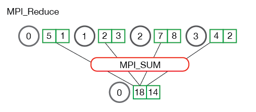
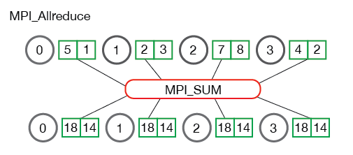
All-reduce is a main component of tensor parallelism where tensors from different parallel processes are summed and synced back to each process. Figure 2 below illustrates the reduce operation where the tensors from processes 0,1,2,3 are summed together for process 0. all-reduce is quite similar in that the tensor is every process is also synced with that final tensor. After all-reduce, all processes are in sync with respect to this tensor. all-reduce is often used to distribute workloads to different processes, then combine them at the end.

For more thorough details on all MPI communications such as scatter, gather, or all-gather, once can check out https://mpitutorial.com/tutorials/mpi-scatter-gather-and-allgather/.

High-Level Illustration

Figure 1 illustrates an overview of tensor parallelism. On the left, we have a GPT architecture. On the right, we have a tensor parallel version where there are two main places for tensor splitting. The first is the attention block where the query, key, and value projection tensors are sharded along the attention head index. That is, each tensor parallel (TP) rank holds the projection parameters only for a subset of attention heads. At first glance, it is not readily clear what modification is required to subsequent operations to make the calculation in TP become identical to the non-TP case. However, we will see the beauty of the multi-head attention in that for tensor parallelism, all operations are identical to wihtout TP (with different input or output tensor shapes), and requires one operation to gather the final attention output tensor with all-reduce.

The feedforward layer is also similar in principle where the two linear layers are sharded, and only requires one all-reduce to gather results for the final feedforward output tensor. Note that we use the same notation as in The Illustrated Attention via Einstein Summation blog.

In the next section, we look at the tensor parallel details for both attention and feedforward layers.

Attention Parallel

Tensor parallelism in the attention layer requires sharding of four model parameters: the query, key, value, and output projection matrices ($P_Q,P_K,P_V,P_O$) respectively. Suppose the original $P_Q^{full}$ is of shape dHk where H is the number of heads. We denote h as the number of heads per GPU where h = H/p and p is the number of GPUs (or tensor parallel size). For each tensor parallel degree (each GPU), $P_Q$ is of size dhk which is reduced from dHk by exactly p times. The same applies for $P_K$ and $P_V$.

All sharded projection parameters within the same process also need to correspond to the same subset of heads for correct TP computation. For instance, if the full model has 4 heads and we want to use 2 GPUs, then the projection matrices for the first GPU can correspond to head index 0,1 whereas the second GPU corresponds to head index 2,3. This splitting needs to be consistent across all projection tensors. If the first GPU has $P_Q$ with 0th and 1st heads, but $P_O$ from 2nd and 3rd heads, this would lead to an incorrect TP computation.

Once we pre-shard the models, in Figure 2, the computation from x to y happens independently for each process. The all-reduce communication is only required at the end to sum y from all processes. To see that TP yields an identical computation as without-TP, at a high level, we can observe that since h axis are retained from Q,K,V after projections, and the reduction over the h axis only occurs at the final output projection $P_O$.

Since for each TP degree, we sum over the h axis that only has a subset of heads, we simply need to sum over all the subsets from all processes to obtain the identical computation as in the non-TP case!

The tensor parallelism in $P_Q,P_K,P_V$ are what we refer to as output parallel, or column parallel. In contrast, the parallelism in $P_O$ is an input parallel.

MLP Parallel

Now that we are familiar with output and input parallel projections, understanding the MLP tensor parallel is quite simple. In this feedforward layer, we have the mapping $C_{fc}$ from input to the intermediate feature which expands the feature dimension from d to 4d. Another mapping $C_{proj}$ maps back the intermediate feature to the output with the feature dimension d.

In order to do tensor parallel, we use similar principles as in the attention tensor parallel where $C_{fc}$ uses output parallel, which in effect, results in the the intermediate feature $x_{inter}$ corresponding a subset of heads. Then, $C_{proj}$ reduces over the head dimension, which again is reduced over all TP degrees to produce the correct output.