The Essense of Global Convolution Models
There are recent exciting developments of AI models for sub-quadratic long context modeling involving the use of global convolutions, ranging from Structured State Space Models (S4) (Gu et al., 2022) (Gu et al., 2022), Gated State Spaces (GSS) (Mehta et al., 2023), H3 (Fu et al., 2023), and most recently, Hyena models (Poli et al., 2023; Nguyen et al., 2023). In this blog post, we will attempt to provide a unified perspective on these models and show how they are related to each other. We will also provide a background on necessary topics, including convolution, fast fourier transform, state space models, and attention.
Prelude
Throughout this blog post, the common goal is to understand how various models define context operators. In the single feature dimension case, given a sequence \(\{ u_i \}_{i=0}^{L}, u_i \in \mathbb{R}\)1, we are interested in effective ways to build a contextualized representation \(y_j \in \mathbb{R}\) that captures the context \(\{u_i\}_{i=0}^j\), which is the input up to time \(j\). A good context representation \(y_j\) can have significant implications. For instance, it can allow us to predict the next time step more accurately, which is useful for various tasks such as forecasting or language modeling.

Attention (Vaswani et al., 2017), for instance, is a popular context operator where \(y_j\) is a weighted sum of the input sequence \(\{u_i\}_{i=0}^j\), based on an input-dependent weight \(A_{ij}\) computed from softmax over dot product between each token and every other tokens in the past. In a vector form, we can also view attention as \(\vec{y} = A \vec{u}\). In general, an context operator can be of any form \(\vec{y} = f(\vec{u})\) where \(f\) is a function. In this blog post, we will see a global convolution operator can be an effective operator \(f\), which builds contextual representation in a global way by aggregating information from all input positions. This is in contrast to short or local convolution where the kernel is of fixed length, popular in convolutional neural networks. The global convolution kernel can also depend on data itself, giving rise of implicit convolution kernels.
Notation
We use the following notations throughout the blog post:
- We interchangeably think of different points along the sequence as time or spatial dimension. For instance, we can think of \(u_i\) as the input at time \(i\) or the input at position \(i\).
- We use \(T\), \(L\), or sometimes \(N\) to denote the sequence length.
- \(\odot\) represents either element-wise multiplication or einstein summation when appropriate.
- \(\mathbf{a} * \mathbf{b}\) denotes the convolution of two vectors \(\mathbf{a}\) and \(\mathbf{b}\). In this post, we primarily deal typically deal with convolution of equal length vectors.
- We either use boldface \(\mathbf{a}\) or \(\vec{a}\) to denote a vector.
Background
The goal for this blog post is to be self-contained and accessible to the broader audience. We will cover background necessary to deeply understand related convolution models and how they compare and connect with transformer’s attention. For instance, we cover the core idea and derivation of convolution theorem and Fast Fourier Transform (FFT), which is at the heart of being able to do long range model with log linear computation. We provide background section on orthonomal basis in function space, which will be important to understand the construction of HiPPO matrix for continuous-time input memorization problem with state space models. We will also cover einstein summation, as it provides a convenient way to tie different operations together under general (linear) tensor operations and is used throughout the blog post. We will also briefly cover transformers attention and its linear version, which provides connection to RNNs and the recurrence nature of state space models.
If you are already familiar with certain topics, feel free to skip. Below outlines the recommended background for each of the convolution models so that one can decide what to focus on.
- HiPPO Framework: requires background A, B, C
- S4: requires background A and C and understanding of HiPPO framework
- H3: requires background A, C and understanding of HiPPO matrix and S4
- Hyena: requires background A. All background topics recommended.
A. Convolution Theorem and Fast Fourier Transform
In this section, we will cover the following topics:
- The concept of convolution, including some illustration and examples of convolution such as the probability distribution interpretation: the density of random variables \(X + Y\) is the convolution of the density \(p_X\) and \(p_Y\).
- Discrete Fourier transform as a way to convert time-domain signal to frequency domain signal, and vice versa.
- Fast Fourier transform as a way to compute the Discrete Fourier transform efficiently.
- Convolution theorem, which states that convolution in time domain is equivalent to multiplication in frequency domain.
What is a Convolution?
Let us consider two N-dimensional vectors \(\mathbf{a}, \mathbf{b} \in \mathbb{R}^N\)2. The convolution of the two vectors, denoted as \(\mathbf{a} * \mathbf{b}\) is defined as:
\[\begin{align*} c_i = (\mathbf{a} * \mathbf{b})_m &= \sum_{n=0}^{N-1} a_n b_{m-n} \\ \end{align*}\]In this notation, we implicitly assume that \(a_n\) or \(b_n\) where \(n \not \in \{0, \dots, N-1\}\) is undefined and is treated as \(0\).
High-Level Intuition
We can see convolution as a way to combine two signals. The first signal is the convolution kernel \(\mathbf{a}\) and the second signal is the input signal \(\mathbf{b}\) (or vice versa since the operation is commutative). The approach of combining signals in convolution is such that for the output \({c}_m\) gather signals from all input pairs \(\{a_{m-n}, b_m\}\) whose indicies add up to \(m\) exactly.
To make it more concrete, let’s expand this out with \(N=4\).
\[\begin{align*} c_0 &= a_0 b_0 \\ c_1 &= a_0 b_1 + a_1 b_0 \\ c_2 &= a_0 b_2 + a_1 b_1 + a_2 b_0 \\ c_3 &= a_0 b_3 + a_1 b_2 + a_2 b_1 + a_3 b_0 \\ c_4 &= a_1 b_3 + a_2 b_2 + a_3 b_1 \\ c_5 &= a_2 b_3 + a_3 b_2 \\ c_6 &= a_3 b_3 \\ \end{align*}\]where we note that \(a_j\) or \(b_j\) are treated as \(0\) for \(j \not \in \{0, \dots, N-1 \}\). We can see that, for instance, \(c_2\) is the sum of \(a_0 b_2\) and \(a_1 b_1\) and \(a_2 b_0\), where the indicies add up to \(2\).

We can also write convolution as a matrix multiplication:
\[\mathbf{c} = \begin{pmatrix} c_0 \\ c_1 \\ c_2 \\ c_3 \\ c_4 \\ c_5 \\ c_6 \\ \end{pmatrix} = \begin{pmatrix} a_0 & 0 & 0 & 0 \\ a_1 & a_0 & 0 & 0 \\ a_2 & a_1 & a_0 & 0 \\ a_3 & a_2 & a_1 & a_0 \\ 0 & a_3 & a_2 & a_1 \\ 0 & 0 & a_3 & a_2 \\ 0 & 0 & 0 & a_3 \\ \end{pmatrix} \begin{pmatrix} b_0 \\ b_1 \\ b_2 \\ b_3 \\ \end{pmatrix} \tag{Convolution}\]or
\[\mathbf{c} = S_a \mathbf{b}\]where \(S_a\) is the convolution matrix representation of vector \(\mathbf{a}\). We observe that \(S_a\) is Toeplitz3, meaning that it each diagonal has constant values from left to right. Since the convolution operator is commutative (\(\mathbf{a} * \mathbf{b} = \mathbf{b} * \mathbf{a}\)), we also have \(\mathbf{c} = S_b \mathbf{a}\) where \(S_b\) is the convolution matrix representation of vector \(\mathbf{b}\).

I included a Colab notebook to visualize the kernel and its matrix representation here.
Causal vs Non-Causal Convolution
Let’s take a look in the case where \(a_n\) have non-zero values where \(n < 0\). Again, let’s use \(N=4\) for simplicity.
\[\begin{align*} c_0 &= a_{-4} b_0 + a_{-3} b_1 + a_{-2} b_2 + a_{-1} b_1 + \textcolor{red}{a_0 b_0} + a_1 b_{-1} + a_2 b_{-2} + a_3 b_{-3} \\ c_1 &= a_{-4} b_1 + a_{-3} b_2 + a_{-2} b_3 + a_{-1} b_2 + \textcolor{red}{a_0 b_1} + \textcolor{red}{a_1 b_0} + a_2 b_{-1} + a_3 b_{-2} \\ c_2 &= a_{-4} b_2 + a_{-3} b_3 + a_{-2} b_4 + a_{-1} b_3 + \textcolor{red}{a_0 b_2} + \textcolor{red}{a_1 b_1} + \textcolor{red}{a_2 b_0} + a_3 b_{-1} \\ \vdots & \end{align*}\]Observe that if \(a_{n} \ne 0\) for \(n < 0\), then, for example, \(c_2\) gets the contribution from \(a_{-3}b_{3}\) where \(b_3\) is an input signal from a future time step. If we would like to perform causal modeling where the output of the current time step is influenced only by current and previous time steps (and not future steps), all \(a_n\) for \(n < 0\) must be \(0\).
In general, due to how we index the inputs where \(a_{n} = 0\) for \(n < 0\) in the original definition, this results in the convolution being causal, which means that the signal \(c_i\) can only depend on input at time \(i\) or before. This is because if there is a term \(b_{i+m}\) for \(m>0\) that contributes to \(c_i\), the corresponding term from \(\mathbf{a}\) is \(a_{-m}\) which is zero (which makes \(b_{i+m}a_{-m} = 0\)).
In addition, throughout this blog post, we are mainly interested in mapping an input signal \(\mathbf{b}\) to and output \(\mathbf{c}\) on the same time domain \(t = 0, \dots, T-1\), in which case we can use the truncated version where \(c_m\) are only defined for \(m \in \{0, \dots, T-1\}\), implying that the corresponding Toeplitz matrix is square and is lower diagonal.
\[\mathbf{c} = \begin{pmatrix} c_0 \\ c_1 \\ c_2 \\ c_3 \\ \end{pmatrix} = \begin{pmatrix} a_0 & 0 & 0 & 0 \\ a_1 & a_0 & 0 & 0 \\ a_2 & a_1 & a_0 & 0 \\ a_3 & a_2 & a_1 & a_0 \\ \end{pmatrix} \begin{pmatrix} b_0 \\ b_1 \\ b_2 \\ b_3 \\ \end{pmatrix}\]Examples of Convolution
We look at a few cases of convolution to develop some intuition. First, let’s consider random variables \(X\) and \(Y\) corresponding to rolling two dice. The probability distribution of \(X\) (or \(Y\)) are:
\[\begin{align*} p_X(x) &= \begin{cases} \frac{1}{6} & x \in \{1, 2, 3, 4, 5, 6\} \\ 0 & \text{otherwise} \end{cases} \end{align*}\]The probability distribution of \(Z = X + Y\) requires summing over all possible combinations of \(X=x\) and \(Y=y\) such that \(x+y = z\). That is, if \(X=x\), \(Y\) must be \(y=z-x\). Therefore, the probability distribution of \(Z\) is exactly the convolution between \(p_X\) and \(p_Y\):
\[\begin{align*} p_Z(z) &= \sum_{x=1}^6 p_X(x) p_Y(z-x) \\ &= p_X * p_Y \end{align*}\]This is one of examples where convolution shows up quite natarually when we deal of probability. Below, we show the illustration of the convolution results, for both a fair die scenario and an unfair one.

Extras: Convolution of Functions
The convolution of two functions \(f\) and \(g\) is the continuous case of the discrete version and is defined as:
\[(f * g)(t) = \int_{-\infty}^{\infty} f(\tau) g(t - \tau) d\tau\]Similar to the discrete case, if we have two random variables \(X\) and \(Y\) with probability density functions \(P_X\) and \(P_Y\) respectively, then the probability density of \(Z = X + Y\) entails integrating all possible \(X=x\) and \(Y=y\) such that \(x+y = z\). That is, if \(X=x\), \(Y\) must be \(y=z-x\). Therefore, the probability density of \(Z\) is:
\[\begin{align*} p_Z(z) &= \int_{-\infty}^\infty p_X(x) p_Y(z-x) dx \\ \end{align*}\]which is the exactly the convolution \(p_X * p_Y\).
Another example entails a convolution of a function and a Dirac delta. The Dirac delta function is defined as:
\[\delta(t) = \begin{cases} \infty & t = 0 \\ 0 & t \neq 0 \end{cases}\]and
\[\int_{-\infty}^{\infty} \delta(t) dt = 1\]The Dirac delta function is a special function that is zero everywhere4 except at \(t=0\), where it is infinite. However, the integral of the function is \(1\), which implies that we can think of Dirac delta function can be thought of as a probability distribution that is entirely concentrated at \(t=0\).
Next, let’s consider the convolution of the Dirac delta function with another function \(f\):
\[\begin{align*} (f * \delta)(t) &= \int_{-\infty}^{\infty} f(\tau) \delta(t - \tau) d\tau \\ &= f(t) \end{align*}\]We can see that the convolution of \(f\) with the Dirac delta function is simply \(f\) itself, or \(\delta\) is an identity function with respect to integration. This is because the Dirac delta function is zero everywhere except when its argument \(t-\tau = 0\). Therefore, the only contribution to the integral comes from \(f(\tau = t)\), which is simply \(f\) itself. We can see in this example that the Dirac delta as a convolution kernel performs an identity operation.
Now, let’s consider the convolution of \(f\) with a shifted Dirac delta function:
\[\begin{align*} (f * \delta(t - \tau))(t) &= \int_{-\infty}^{\infty} f(\tau') \delta(t - \tau - \tau') d\tau' \\ &= f(t - \tau) \end{align*}\]The convolution of \(f\) with a shifted Dirac delta function is simply \(f\) shifted by \(\tau\)! This is because the shifted Dirac delta function is zero everywhere except at \(\tau'=t-\tau\). Therefore, the only contribution to the integral comes from \(f(\tau)\), which is simply \(f\) shifted by \(\tau\).
Discrete Fourier Transform
The Discrete Fourier Transform (DFT) is a mathematical operation used to analyze the frequency components of a discrete signal. Given a discrete sequence of values \(x[n]\) for \(n = 0, 1, 2, \ldots, N-1\), the DFT computes a set of complex coefficients \(X[k]\) for \(k = 0, 1, 2, \ldots, N-1\) that represent the frequency content of the signal. The DFT is defined as:
\[X[k] = \sum_{n=0}^{N-1} x[n] \cdot e^{-i\frac{2\pi}{N}kn}\]Here:
- \(X[k]\) is the DFT coefficient at frequency \(k\).
- \(x[n]\) is the input signal at time index \(n\).
- \(N\) is the total number of samples in the input signal.
- The coefficients are complex and can be interpreted as the coefficients of the sine and cosine components (see more in Fourier Basis).
The original series can be recovered from \(X[k]\) via the inverse DFT (IDFT):
\[x[m] = \frac{1}{N} \sum_{k=0}^{N-1} X[k] \cdot e^{i\frac{2\pi}{N}km}\]To show that \(x[m]\) as can recovered exactly as above, we will make use of the following results for geometric series. For \(r \in \mathbb{C}\) and \(r \neq 1\),
\[\sum_{k=0}^{N-1} r^k = \frac{1 - r^N}{1 - r}\]In this case, \(r = e^{-i\frac{2\pi}{N}(n-m)}\) and \(r^N = e^{-i2\pi(n-m)}\). For \(n \ne m\), the exponent is an integer multiple of \(2\pi\), which means that \(r^N = 1\) and \(\sum_{k=0}^{N-1} r^k = \frac{1 - r^N}{1 - r} = 0\). For \(n = m\), \(r = 1\) and \(\sum_{k=0}^{N-1} r^k = \sum_{k=0}^{N-1} 1 = N\). Therefore, we can concisely write
\[\sum_{k=0}^{N-1} e^{-i\frac{2\pi}{N}k(n-m)} = N \cdot \delta_{n,m}\]where \(\delta_{n,m}\) is the Kronecker delta function, which is \(1\) if \(n=m\) and \(0\) otherwise.
Then, the iDFT becomes:
\[\begin{align*} \frac{1}{N} \sum_{k=0}^{N-1} X[k] \cdot e^{i\frac{2\pi}{N}km} &= \frac{1}{N} \sum_{k=0}^{N-1} \left( \sum_{n=0}^{N-1} x[n] \cdot e^{-i\frac{2\pi}{N}kn} \right) \cdot e^{i\frac{2\pi}{N}km} \\ &= \frac{1}{N} \sum_{n=0}^{N-1} \left( x[n] \cdot \sum_{k=0}^{N-1} e^{-i\frac{2\pi}{N}k(n-m)} \right) \\ &= \frac{1}{N} \sum_{n=0}^{N-1} x[n] \cdot N \cdot \delta_{n,m} \\ &= x[m] \end{align*}\]which means that we recover the original signal \(x[m]\) for \(m = 0, \dots, N-1\) perfectly from the DFT coefficients \(X[k]\). There is no information loss in the DFT operation.
We can think of this as a duality between the spatial domain and the frequency domain. The DFT converts a signal from the spatial domain (\(N\) numbers) to the frequency domain (\(N\) numbers), and the iDFT converts a signal from the frequency domain back to the spatial domain. The DFT and iDFT are inverse operations of each other.
In terms of computational complexity, both DFT and iDFT involves summing \(N\) numbers for each of the \(N\) entries, thus incurs a complexity \(O(N^2)\). Next, we will discuss a way to perform these operations efficiently with log linear complexity (without any approximation!!) by exploiting special structures of the complex exponentials. This is the main idea behind Fast Fourier Transform (FFT).
Fast Fourier Transform
Fast Discrete Fourier Transform or more commonly called Fast Fourier Transform (FFT) is an algorithm that computes the DFT efficiently. The FFT algorithm is based on the divide-and-conquer strategy, and is able to compute the DFT in \(O(N \log N)\) time, which is much faster than the naive \(O(N^2)\) algorithm. We sketch a proof below.
Let’s start with the DFT definition:
\[X[k] = \sum_{n=0}^{N-1} x[n] \cdot e^{-i\frac{2\pi}{N}kn}\]We can rewrite this by splitting into the odd and even terms as:
\[X[k] = \sum_{n=0}^{N/2-1} x[2n] \cdot e^{-i\frac{2\pi}{N}k(2n)} + \sum_{n=0}^{N/2-1} x[2n+1] \cdot e^{-i\frac{2\pi}{N}k(2n+1)}\]We can further rewrite this as:
\[\begin{align*} X[k] &= \sum_{n=0}^{N/2-1} x[2n] \cdot e^{-i\frac{2\pi}{N/2}kn} + e^{-i\frac{2\pi}{N}k} \sum_{n=0}^{N/2-1} x[2n+1] \cdot e^{-i\frac{2\pi}{N/2}kn} \\ &= E_k + e^{-i\frac{2\pi}{N}k} O_k \end{align*}\]We can see that the first term is the DFT of the even terms of \(x\), denoted by \(E_k\), and the second term is the DFT of the odd terms of \(x\), denoted by \(O_k\), multiplied by a complex exponential. The key part is that we also obtain \(X[k + \frac{N}{2}]\) for free once we have \(E_k\) and \(O_k\), due to the identity:
\[X[k + \frac{N}{2}] = E_k - e^{-i\frac{2\pi}{N}k} O_k\]To obtain \(E_k\) (or \(O_k\)), we recursively break up it up into two terms, and so on. Therefore, the computational complexity of DFT to obtain \(X[k]\) consists of the complexity of two DFT of \(N/2\) elements plus \(O(1)\) operations, amortized by two, since for each \(X[k]\), we also get \(X[k+ \frac{N}{2}]\). This gives us the following recurrence relation:
\[T(N) = \frac{1}{2} \left( 2 T(N/2) + O(1) \right)\]which yields \(T(N) = O(\log N)\). For all \(k\), this results in an \(O(N \log N)\) algorithm for DFT.
The Convolution Theorem
In this section, we will show that a convolution of two vectors can be seen as a multiplication of their Fourier transforms. This is known as the convolution theorem. We will show this in the discrete case. The continuous case extends naturally by replacing the summation with an integral (with exchange of order justified by Fubini’s theorem).
The convolution of two sequences \(\mathbf{a}\) and \(\mathbf{b}\) is defined as:
\[\begin{align*} \mathbf{c}_m = (\mathbf{a} * \mathbf{b})_m &= \sum_{n=0}^{N-1} a_n b_{m-n} \\ \end{align*}\]The Fourier transform of a sequence \(\mathbf{a}\) is defined as:
\[\begin{align*} \mathbf{A}_k = \left(\mathcal{F}(\mathbf{a}) \right)_k &= \sum_{n=0}^{N-1} a_n e^{-i\frac{2\pi}{N}kn} \\ \end{align*}\]Then,
\[\begin{align*} \left( \mathcal{F} (\mathbf{a} * \mathbf{b}) \right)_k &= \sum_{m=0}^{N-1} (\mathbf{a} * \mathbf{b})_m e^{-i\frac{2\pi}{N}km} \\ &= \sum_{m=0}^{N-1} \left( \sum_{n=0}^{N-1} a_n b_{m-n} \right) e^{-i\frac{2\pi}{N}km} \\ &= \sum_{n=0}^{N-1} \sum_{m=0}^{N-1} a_n e^{-i\frac{2\pi}{N}kn} b_{m-n} e^{-i\frac{2\pi}{N}k(m-n)} \\ &= \sum_{n=0}^{N-1} a_n e^{-i\frac{2\pi}{N}kn} \sum_{m=0}^{N-1} b_{m-n} e^{-i\frac{2\pi}{N}k(m-n)} \\ &= \sum_{n=0}^{N-1} a_n e^{-i\frac{2\pi}{N}kn} \sum_{s=-n}^{N-1-n} b_s e^{-i\frac{2\pi}{N}ks} \\ &= \left( \sum_{n=0}^{N-1} a_n e^{-i\frac{2\pi}{N}kn} \right) \left( \sum_{s=0}^{N-1} b_s e^{-i\frac{2\pi}{N}ks} \right)\\ &= \mathbf{A}_k \cdot \mathbf{B}_k \\ &= \mathcal{F}(\mathbf{a}) \cdot \mathcal{F}(\mathbf{b}) \end{align*}\]where we exchange variable \(s = m-n\) and the fact that \(b_s = 0\) for \(0 < s < N-1\), so the sum \(\sum_{s=-n}^{N-1-n} b_n \cdot \xi\) is the same as \(\sum_{s=0}^{N-1} b_n \cdot \xi\). The proof can also be done simpler by consider the summation from \(-\infty\) to \(\infty\) where values beyond its support are zero.
Extras: Continuous Case of Convolution Theorem
In the continuous case involving convolution of two functions \(f\) and \(g\), we also provide a proof sketch below.
The convolution of two functions is defined as:
\[(f * g)(t) = \int_{-\infty}^{\infty} f(\tau) g(t - \tau) d\tau\]Then, the Fourier transform of the convolution is:
\[\begin{align*} \mathcal{F}[f * g](\omega) &= \int_{-\infty}^{\infty} (f * g)(t) e^{-i \omega t} dt \\ &= \int_{-\infty}^{\infty} \left( \int_{-\infty}^{\infty} f(\tau) g(t - \tau) d\tau \right) e^{-i \omega t} dt \\ &= \int_{-\infty}^{\infty} f(\tau) \left( \int_{-\infty}^{\infty} g(t - \tau) e^{-i \omega t} dt \right) d\tau \\ &= \int_{-\infty}^{\infty} f(\tau) \left( \int_{-\infty}^{\infty} g(t) e^{-i \omega (t + \tau)} dt \right) d\tau \\ &= \left( \int_{-\infty}^{\infty} f(\tau) e^{-i \omega \tau} d\tau \right) \cdot \left( \int_{-\infty}^{\infty} g(t) e^{-i \omega t} dt \right) \\ &= \mathcal{F}[f](\omega) \cdot \mathcal{F}[g](\omega) \end{align*}\]Or in other words,
\[(f*g)(w) = \mathcal{F}^{-1}[\mathcal{F}[f](\omega) \cdot \mathcal{F}[g](\omega)](w)\]Convolution Theorem + FFT = Log Linear Convolution
To recap, the implication of the convolution theorem is that if we want to perform a convolution of long signals \(f(t)\) and \(g(t)\), which naively would incur \(O(N^2)\) computational complexity, we can reduce it to \(O(N \log N)\) without any approximation. Below are the steps:
- Compute the Fourier transform of vectors \(a\) and \(v\), each of length \(N\), which incures \(O(N \log N)\) via Fast Fourier Transform. Here, we obtain the frequency components \(A\) and \(B\), each of length \(N\).
- Multiply the Fourier transforms of two vectors \(A\) and \(B\), incurring \(O(N)\), and finally compute the inverse Fourier transform of \(A \cdot B\), which incurs another \(O(N \log N)\).
- In total, the convolution can be done in \(O(N \log N)\) via Fast Fourier Transform and the Convolution Theorem, instead of the usual \(O(N^2)\). Magic!
- This sub-quadratic behavior allows fast long range modeling, and is the foundation of convolution models such as S4, S4d, GSS, H3, and Hyena.
B. Orthonormal Basis in Function Space
We turn our attention to a vector space whose elements are functions. A special kind of such vector space we will consider is a Hilbert space5 \(\mathcal{H}\) that is equipped with a countable and dense orthonormal basis6 \(\{ g_n \}_{n=0}^\infty\). In essence, a Hilbert space provides a notion of projections and distance via its inner product \(\langle f, h \rangle\) and the induced norm \(\| f \| = \sqrt{\langle f, f \rangle}\). Further, a Hilbert space has a completeness property, meaning that any sequence of elements in \(\mathcal{H}\) that draws progressively closer together actually converge within the space. As example of such a Hilbert space is the space of square integrable functions on an interval \(L^2[a,b]\), with a corresponding inner product
\[\langle f, g \rangle = \int_a^b f(x)^* g(x) \cdot w(x) dx\]where \(f(x)^*\) denotes the complex conjugate of \(f\). The function \(w(x)\) corresponds to the weight of different points in the interval which reflects the measure that the inner product is defined on.7 For instance, we may want to weigh points far away with smaller weights. Different weight \(w(x)\) used in the integral above (or different measure) will give rise to a different inner product, which in turn defines a different notion of orthogonality and distance in the associated Hilbert space.
The power of the dense orthonormal basis \(\mathcal{G}\) is that it allows us to represent any function in the Hilbert space using a linear combination of the basis elements. That is, for any function \(u(t) \in \mathcal{H}\), there exists coefficients \(\{ c_n \}_{n=1}^\infty\) such that:
\[u(t) = \sum_{n=1}^{\infty} c_n g_n(t)\]That is, in the orthonormal basis \(\mathcal{G}\), a function \(u\) can be represented as simply an infinite sequence \(\{c_n\}_{n=1}^\infty\). 8 It is quite profound that an entire function whose domain consists of uncountably many numbers can be described by a countable set of numbers, the coefficients of the respective basis.
We can also think of the partial sum \(u_m(t) = \sum_{n=1}^{m} c_n g_n(t)\) as an approximation of the function \(u(t)\), where the approximation gets better as \(m \to \infty\) (where the convergence is in the norm9). Therefore, a finite vector \((c_1, c_2, .., c_m)\) can also be used to approximately represent an entire function where the approximation gets better as \(m\) is larger. This concept is used widely for compression of signals such as audio, images, and videos.
While this representation ensures approximation, it does not directly offer a method to find \(c_n\) for a given \(u(t)\). The key lies in the orthogonality of the basis. The set \(\{ g_n \}\) is orthonormal, implying \(\langle g_m, g_n \rangle = \delta_{m,n}\), where \(\delta_{m,n}\) is the Kronecker delta, a function that returns 1 when \(m = n\) and 0 otherwise. This orthogonality simplifies our task of finding coefficients to taking inner products, where we extract the coefficient of \(g_n\) via:
\[\begin{align*} \langle u(t), g_n(t) \rangle &= \langle \sum_{m=1}^{\infty} c_m g_m(t), g_n(t) \rangle \\ &= \sum_{m=1}^{\infty} c_m \langle g_m(t), g_n(t) \rangle \\ &= \sum_{m=1}^{\infty} c_m \delta_{m,n} \\ &= c_n \end{align*}\]This filtering property, intrinsic to orthonormal bases, ensures that we isolate each coefficient efficiently.
Based on the weight function \(w(x)\) and the subspace of functions we operate on, the orthonormal basis can be different. For instance, for uniform weight \(w\) on an interval, the Legendre polynomials form an orthonormal basis. For periodic functions with uniform weight \(w\) on an interval, the Fourier series form an orthonormal basis. For an exponentially decaying weight \(w\), the Laguerre polynomials form an orthonormal basis. We will discuss these three examples below.
Example 1: Legendre Polynomials as Orthonormal Basis on Uniform Measure
The space of square-integrable functions over the interval \([-1, 1]\), denoted by \(L^2[-1,1]\), is an example of a Hilbert space. The inner product is defined as \(\langle f,g \rangle = \int f(x) \cdot g(x) dx\). In this space, the Legendre polynomials form a countable orthonormal basis.
The Legendre Polynomials offer a rich tapestry of function spaces that play a pivotal role across mathematics and physics. Originating from the studies of celestial mechanics by Adrien-Marie Legendre, these polynomials have since been embraced in various applications spanning from quantum mechanics to approximation theory.
Definition: The \(n^{th}\) Legendre polynomial, denoted \(P_n(x)\), is given by Rodrigues’ formula:
\[P_n(x) = \frac{1}{2^n n!} \frac{d^n}{dx^n} \left[ (x^2 - 1)^n \right]\]More concretely,
\[\begin{align*} P_0(x) &= 1 \\ P_1(x) &= x \\ P_2(x) &= \frac{1}{2} (3x^2 - 1) \\ P_3(x) &= \frac{1}{2} (5x^3 - 3x) \\ &\ .. \end{align*}\]These polynomials are orthogonal on the interval \([-1,1]\) with respect to the weight function \(w(x) = 1\). In other words:
\[\int_{-1}^{1} P_m(x) P_n(x) dx = \frac{2}{2n+1} \delta_{m,n}\]where \(\delta_{m,n}\) is the Kronecker delta function.
The example above can be extended to a Hilbert space defined on \(L^2[a,b]\), where the orthonormal basis functions can be derived as follows.
We introduce a linear change of variables to adapt \([-1,1]\) to the interval \([a,b]\). By defining a new variable \(y\) such that \(y = \frac{2(x - a)}{b - a} - 1\), we transform the interval \([a,b]\) to \([-1,1]\). The Legendre polynomials on the interval \([a,b]\) are then expressed as \(P_n\left( \frac{2(x - a)}{b - a} - 1 \right)\). Define \(\tilde{P}_n(x)\) as a normalized Legendre polynomial, together with \(dy = \frac{2}{b-a} dx\) and \(\int P_m P_n dx = \delta_{m,n}\), we have:
\[\tilde{P}_n(x) = \sqrt{\frac{2n+1}{b-a}} P_n\left( \frac{2(x - a)}{b - a} - 1 \right)\]Example 2: Fourier Basis for Periodic Functions
On \(L^2[-L,L]\) with the inner product \(\langle f,g \rangle = \frac{1}{2L} \int_{-L}^{L} f(x)^* g(x) dx\) where \(^*\) denotes complex conjugate, the Fourier basis is an orthonormal basis when applied to periodic functions.10
The Fourier series representation of a periodic function \(f(x)\) over the interval \([-L,L]\) is given by:
\[f(x) = \sum_{n=-\infty}^{\infty} c_n e^{i\frac{2\pi n}{2L}x}\]where \(c_n\) are the Fourier coefficients of the basis elements \(f_n = e^{i\frac{2\pi n}{2L}x}\), computed as:
\[c_n = \langle e^{i\frac{2\pi n}{2L}x}, f(x) \rangle = \frac{1}{2L} \int_{-L}^{L} e^{-i\frac{2\pi n}{2L}x} f(x) dx\]We can extract out the coefficient \(c_n\) from the inner product with \(f_n\) because for distinct integers \(m\) and \(n\), the basis functions \(f_n\) and \(f_m\) are orthogonal on the interval \([-L,L]\). Their inner product is:
\[\begin{align*} \langle f_n , f_m \rangle &= \frac{1}{2L} \int_{-L}^{L} e^{- i\frac{2\pi m}{2L}x} e^{i\frac{2\pi n}{2L}x} dx \\ &= \frac{1}{2L} \int_{-L}^{L} e^{i\frac{2\pi (n-m)}{2L}x} dx \\ &= \frac{1}{2L} \left[ \frac{1}{i\frac{2\pi (n-m)}{2L}} e^{i\frac{2\pi (n-m)}{2L}x} \right]_{-L}^{L} \\ &= \frac{1}{2L} \frac{1}{i\pi (n-m)} \left[ e^{i\pi (n-m)} - e^{-i\pi (n-m)} \right] \\ &= \frac{1}{2L} \frac{1}{i\pi (n-m)} \left[ (-1)^{n-m} - (-1)^{n-m} \right] \\ &= 0. \end{align*}\]For \(n=m\), we have \(\frac{1}{2L} \int_{-L}^{L} e^{- i\frac{2\pi m}{2L}x} e^{i\frac{2\pi m}{2L}x} dx = \frac{1}{2L} \int_{-L}^{L} 1 dx = 1\), which is indeed normalized.
How do we interpret complex coefficients?
The complex representation here is a convenient way to express the Fourier basis, but we can also express it in terms of cosine and sine functions which gives us nice physical interpretations. This integer multiples of the base frequency (or simply called harmonics), with arbitrary phase in that frequency controlled by the relative coefficient of the cosine and sine functions.
Expanding \(c_n = a_n + i b_n\) and \(e^{i \omega n x } = \cos(\omega n x) + i \sin(\omega n x)\) where \(\omega = \frac{2 \pi}{2L}\), we have
\[\begin{align*} f(x) &= \sum_{n=-\infty}^{\infty} c_n e^{i \omega n x} \\ &= \sum_{n=-\infty}^{\infty} (a_n + i b_n) (\cos(\omega n x) + i \sin(\omega n x)) \\ &= \sum_{n=-\infty}^{\infty} (a_n \cos(\omega n x) - b_n \sin(\omega n x)) + i \sum_{n=-\infty}^{\infty} (b_n \cos(\omega n x) + a_n \sin(\omega n x)) \end{align*}\]Now, let’s simplify it doing a sum over non-negative \(n\), from \(0\) to \(\infty\). We’ll start with the real part of the function decomposition of \(f\), which is given by:
\[\begin{align*} \text{Re}[f(x)] &= \sum_{n=-\infty}^{\infty} (a_n \cos(\omega n x) - b_n \sin(\omega n x)) \\ &= a_0 + \sum_{n=1}^{\infty} (a_n \cos(\omega n x) - b_n \sin(\omega n x) + \sum_{n=1}^{\infty} (a_{-n} \cos(-\omega n x) - b_{-n} \sin(- \omega n x) \\ &= a_0 + \sum_{n=1}^{\infty} (a_n + a_{-n}) \cos(\omega n x) + (- b_n + b_{-n}) \sin(\omega n x) \\ \end{align*}\]The complex part of the function decomposition of \(f\) is given by:
\[\begin{align*} \text{Im}[f(x)] &= \sum_{n=-\infty}^{\infty} (b_n \cos(\omega n x) + a_n \sin(\omega n x)) \\ &= b_0 + \sum_{n=1}^{\infty} (b_n \cos(\omega n x) + a_n \sin(\omega n x)) + \sum_{n=1}^{\infty} (b_{-n} \cos(-\omega n x) + a_{-n} \sin(- \omega n x) \\ &= b_0 + \sum_{n=1}^{\infty} (b_n + b_{-n}) \cos(\omega n x) + (a_n - a_{-n}) \sin(\omega n x) \\ \end{align*}\]In short, the complex coefficients \(c_n\) is such that their real and imaginary parts are the coefficients of the cosine and sine functions, respectively.
Real-Valued Functions
If the function \(f(x)\) is real, then \(\text{Im}[f(x)] = 0\), which implies that \(b_0 = 0\) and \(a_n = a_{-n}\) and \(b_n = -b_{-n}\). That is, for real \(f\), we do not need to compute the coefficients with respect to negative frequencies due the symmetry.
The simplified components for a real \(f\) becomes:
\[\begin{align*} f(x) &= a_0 + \sum_{n=1}^{\infty} (a_n + a_{-n}) \cos(\omega n x) + (- b_n + b_{-n}) \sin(\omega n x) \\ &= a_0 + 2\sum_{n=1}^{\infty} a_n \cos(\omega n x) - b_n \sin(\omega n x) \\ &= a_0 + 2 \sum_{n=1}^{\infty} \sqrt{a_n^2 + b_n^2} \cos(\omega n x - \phi_n) \\ \end{align*}\]where \(\phi_n = \tan^{-1} \left( \frac{b_n}{a_n} \right)\). In this interpretation, any periodic function is a linear combinarion of cosine waves with integer multiples of the base frequency (or simply called harmonics), with arbitrary phase of that frequency controlled by the relative coefficient of the cosine and sine functions. This is the physical interpretation for a real signal \(f\) we alluded to earlier.
In practice, the complex representation is more convenient to use and has wide adoption. It is also a generalization of the sine and cosine representation that is applicable for both real and complex functions.
Example 3: Laguerre Polynomials as Orthonormal Basis on Expontential Decay Measure
In the context of Hilbert spaces, another example of an orthonormal basis is provided by the Laguerre polynomials. The space of square-integrable functions over the interval \([0, \infty)\), denoted as \(L^2[0, \infty)\), serves as an example where these polynomials form a countable orthonormal basis.
Definition: The \(n^{th}\) Laguerre polynomial, denoted as \(L_n(x)\), can be defined through Rodrigues’ formula:
\[L_n(x) = \frac{e^x}{n!} \frac{d^n}{dx^n} \left(e^{-x}x^n\right)\]In more concrete terms, the first few Laguerre polynomials are as follows:
\[\begin{align*} L_0(x) &= 1 \\ L_1(x) &= 1 - x \\ L_2(x) &= \frac{1}{2}(x^2 - 4x + 2) \\ L_3(x) &= \frac{1}{6}(-x^3 + 9x^2 - 18x + 6) \\ &\vdots \end{align*}\]These polynomials are orthogonal over the interval \([0, \infty)\) with respect to the weight function \(w(x) = e^{-x}\). In other words, they satisfy the following orthogonality condition:
\[\int_{0}^{\infty} L_m(x) L_n(x) e^{-x} dx = \delta_{m,n}\]Here, \(\delta_{m,n}\) is the Kronecker delta function.
We can see that a different weight function, or a different measure, would give rise to a different set of orthonormal basis functions. This is a powerful concept that we will revisit later in the context of convolution models, especially in the construct of the HiPPO matrix.
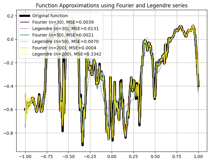
Examples: Approximating Data with Legendre vs. Fourier Basis
We show a few examples here where we use Legendre and Fourier bases to approximate functions with finite number of basis elements \(n\). See a Colab notebook for code and more examples here for the code.
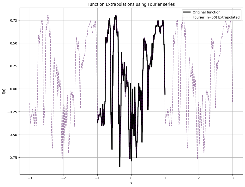
If we extrapolate the data outside the original domain, for Fourier series, the pattern repeats periodically. This can also be shown analytically by observing that for any \(x \in [-L,L]\), we have \(f(x) = f(x + 2L)\) in the Fourier representation.
C. State Space Models
State space models are a class of models used to describe the time evolution of systems. They are widely used in many fields, including control theory, signal processing, and machine learning. In this section, we will give a brief introduction to state space models, and show how they can be used to model complex dynamics.
In the continuous time scenario, linear state space models can be written as matrix-vector multiplications where the \(N\)-dimensional state vector \(\mathbf{x}(t)\) evolves over time \(t\) according to the following differential equation:
\[\begin{align*} \frac{d}{dt} \mathbf{x}(t) &= A \mathbf{x}(t) + B \mathbf{u}(t) \\ \mathbf{y}(t) &= C \mathbf{x}(t) + D \mathbf{u}(t) = C \mathbf{x}(t) \end{align*}\]where \(u(t) \in \mathbb{R}\), \(A\) is an \(N \times N\) matrix, \(B\) is \(N \times 1\), and \(C\) is \(1 \times N\). \(\mathbf{u}\) is usually called the input vector, and \(\mathbf{y}\) is the output vector. In most cases \(D\) is assumed to be \(0\).
Recurrent View of State Space Models
In the discretized case, the evolution goes from time step \(t=k-1\) to \(t=k\), instead of infinitesimal step in the continuous time dynamics \(t\) to \(t + dt\). We can approximate \(x_k\) by either using the derivative at \(k\), or also the average of the derivative at \(k\) and \(k-1\) for better numerical stability (bilinear/trapezoid method). With step size \(\Delta\),
\[x_{k} \approx x_{k-1} + \frac{\Delta}{2} (x'_{k} + x'_{k-1}) + O(\Delta^2)\]Together with the state space equations, we can show that
\[\begin{align*} x_{k} &= (I - \frac{\Delta}{2} A)^{-1} (I + \frac{\Delta}{2} A) x_{k-1} + \frac{\Delta}{2} B (I - \frac{\Delta}{2} A)^{-1} u_k \\ & \ \text{or more succinctly}\\ x_{k} &= \bar{A} x_{k-1} + \bar{B} u_k \\ y_k &= C x_k \end{align*}\]That is, we can obtain the current state \(x_k\) given the the input \(u_k\) and only past state \(x_{k-1}\), without needing to know the previous states or inputs. This is a recurrent property that is useful during inference since it incurs \(O(1)\) compute complexity without dependency of the context length. This is quite different from attention where we need to use cached key and value to predict the next step, which incurs \(O(L)\) memory IO and compute during incremental decoding.

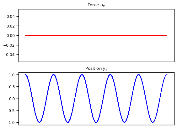
Example: Harmonic Oscillator
Let’s develop some intuition for what state space models can do. We will consider a simple example of a spring attached to a mass \(m\). The spring has a spring constant \(k\), and the mass is attached to a wall. The mass is also subject to a force \(u(t)\).
The dynamics of the system is described by the following differential equation:
\[m y''(t) = -k y(t) + u(t)\]where \(y(t)\) is the displacement from equilibrium of the mass at time \(t\). We know that in the case of \(u(t) = 0\), this should be a simple harmonic oscillator where the solutions are pure sine wave with certain phase (depending on the initial position and velocity). Let’s see how well we can model this system using a state space model.
The key is how we define the state \(\mathbf{x}\). Let \(v(t) = \frac{dy}{dt}\) denote the velocity. In this case, we can see that the differential equation above can be written as:
\[v'(t) = - \frac{k}{m} y(t) + \frac{1}{m} u(t)\]If we define the state as
\[x = \begin{bmatrix} y \\ v \end{bmatrix}\]then we can describe the differential equation with state space model as:
\[\mathbf{x}'(t) = \begin{bmatrix} y'(t) \\ v'(t) \end{bmatrix} = \begin{bmatrix} 0 & 1 \\ -\frac{k}{m} & 0 \\ \end{bmatrix} \begin{bmatrix} y(t) \\ v(t) \end{bmatrix} + \begin{bmatrix} 0 \\ \frac{1}{m} \\ \end{bmatrix} u(t)\]The upper row simply says \(y'(t) = v(t)\), the definition of velocity. The lower row says \(v'(t) = -\frac{k}{m} y(t) + \frac{1}{m} u(t)\), exactly the equation for the acceleration. Then, we extract out the position by
\[y(t) = \begin{bmatrix} 1 & 0 \\ \end{bmatrix} \mathbf{x}(t) = C \mathbf{x}(t)\]In this case we use the initial condition such as
\[\mathbf{x}[0] = \begin{bmatrix} 1 \\ 0 \\ \end{bmatrix}\]which corresponds to initial position at $1$ without velocity. We also use \(u(t) = 0\), meaning that no additional force is applied. We can see that the position calculated via the discretized discrete state space follows the sine equation quite perfectly. See the Colab notebook here. Note that we adapted the code given in The Annotated S4 for state space models.
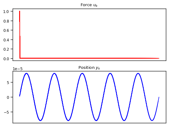
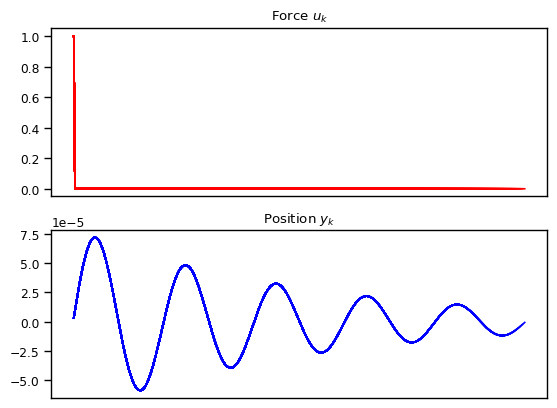
Just for fun, let’s also consider another case where we start from initial position and velocity \(0\), but with \(u[t]\) being something like a Dirac Delta function which injects a fixed momentum at time \(t=0\). In this case, \(u[0] = 1\) and \(u[t] = 0\) for all \(t > 0\). As shown below, the state space models are able to capture the dynamics quite nicely.
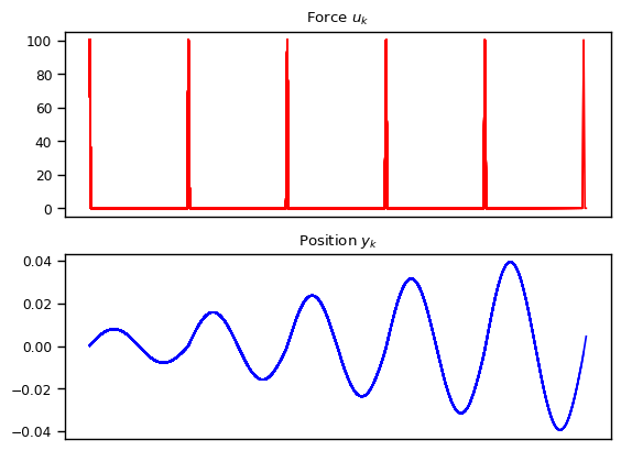
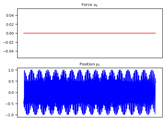
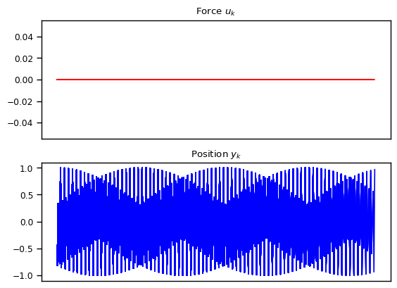
We also explore other variations such as exponentially decay amplitude due to friction and resonance where the external force has the same frequency as the natural frequency. We also show the cases where the numerical approximation can break down resulting in alising effect, once the frequency becomes too high compared to the granularity of the discretization.
What Can We Model With Linear State Space Models?
In general, any linear differential equations can be framed as a linear state space. This excludes some dynamics; for instance, celestial mechanics, where the gravitational force is proportional to the inverse square of the distance between the two bodies, cannot be modeled with a linear state space.
Convolution View of State Space Models
Now let’s think about how we can process a vector input \(\mathbf{u} = \{ u_k \}_{k=0}^L\) to obtain an output \(\{y_k\}_{k=0}^L\) in batch. Due to the recurrence relations, we can write the output \(y_k\) as
\[\begin{align*} y_k &= \sum_{i=0}^{k} \bar{C} \bar{A}^{k-i} \bar{B} u_i + \bar{C} \bar{A}^k x_0 \\ y_k &= \sum_{i=0}^{k} \bar{K}_{k-i} u_i + 0 \\ \end{align*}\]where \(\bar{K}_n = \bar{C} \bar{A}^n \bar{B}\) and \(x_0\) is the initial state, which is often taken to be zero. In this form, we see that \(y_k\) is a convolution between the L-dimensional vector \(\mathbf{\bar{K}}\) and the input vector \(\mathbf{u}\). It means that we can think of the state space model as a convolution model, where the convolution kernel is \(\mathbf{\bar{K}}\). This unrolled view is useful to process the entire input sequence, either during inference or training.
That is, if we have a sequence of length \(L\) as an input, once if we the kernel \(\mathbf{\bar{K}}\), we can compute the entire output \(\mathbf{y}\) in \(O(L \log L)\) time due to the convolution theorem + FFT. The batched operation is important for training as well as initial processing of input sequence during inference.
SSM for Sequence Modeling
Now, you may wonder what would be the matrices \(A\), \(B\), \(C\) that we should use? Remember from our earlier examples for the harmonic oscillator that the matrix \(A\) controls the evolution of the dynamical system. How should we construct or interpret such a system to model something such as language modeling or time series forecasting? In a later section, we discuss the HiPPO matrix, which defines a type of matrix \(A\) that can be used to model long range dependencies.
D. Einstein Summation for General Tensor Operations
We cover a brief introduction to Einstein summation, which is a concise notation for tensor operations. We will use this notation to describe attention or other tensor operations in a concise manner.
Let’s consider the attention weight between query tensor \(Q\) and key tensor \(K\). The query tensor is of shape \(Q_{bhnk}\) where \(b\) is the batch index, \(h\) is the head index, \(n\) is the query length index, and \(k\) is the head dimension index. The key tensor is of shape \(K_{bhmk}\) where \(m\) is the key length index. The attention weight tensor is of shape \(A_{bhnm}\).
The attention weight tensor, before softmax, can be described in various ways such as
\[\begin{align*} A_{bhnm} &= \sum_{k} Q_{bhnk} K_{bhmk} \tag{explicit sum over $k$} \\ A_{bhnm} &= \sum Q_{bhnk} K_{bhmk} \tag{implicit sum over $k$} \\ A_{bhnm} &= Q_{bhnk} K_{bhmk} \tag{what Einstein would write} \\ A_{bhnm} &= \langle Q_{bhnk} , K_{bhmk} \rangle \tag{inner product notation} \\ A &= \langle Q, K \rangle \end{align*}\]In all of the notations above, we are summing over the head dimension \(k\), which is the dimension that we are reducing. The sum over \(k\) need not be explicitly mentioned if the output dimension is specified. That is, since \(A_{bhnm}\) does not contain \(k\), it implies that the output is the result of reduction over \(k\). Since this is akin to inner product over \(k\) where all other axes are broadcasted, we can write it as \(\langle Q, K \rangle\) for simplicity.
Below are examples of various einsum operations. For more details on attention with einsum, see a separate blog post The Illustrated Attention via Einstein Summation.

E. Attention and Linear Attention
In this section, we will describe both attention (Vaswani et al., 2017) and linear attention (Katharopoulos et al., 2020). Let \(\sigma\) be a non linear operator where we may denote \(\sigma_L\) to emphasize that the operation \(\sigma\) is non linear over axis \(L\). We use the same notation as in the last section where both \(k,v\) are the head dimension index for key and value. We drop the batch dimension for simplicity.
With this notation, the attention operation (Vaswani et al., 2017) can be written as
\[\begin{align*} O_{hnv} &= \sum_{m=0}^n V_{hmv} \ \sigma_m \left( \sum_{k} Q_{hnk} K_{hmk} \right) \\ &= \sum_{m=0}^n V_{hmv} \ \sigma_m \left( A_{hmn} \right) \\ &= \sum_{m=0}^n V_{hmv} \ W_{hmn} \end{align*}\]The causality of attention is reflected in the summation over \(m\), which is the key length. That is, the query at position \(n\) can only attend to the keys up to position \(n\). Note that we omit the multiplicative term \(\frac{1}{\sqrt{d}}\) for \(\sum_{k=1}^d Q_{hnk} K_{hmk}\) for simplicity. More details on attention can be found in The Illustrated Attention via Einstein Summation.
Linear Attention
If \(\sigma_m\) is an identity function11, we can rearrange things where \(K\) and \(V\) equivalently interact with each other first. That is,
\[\begin{align*} O_{hnv} &= \sum_{m=0}^n V_{hmv} \left( \sum_{k} Q_{hnk} K_{hmk} \right) \\ &= \sum_k Q_{hnk} \left( \sum_{m=0}^n V_{hmv} K_{hmk} \right) \end{align*}\]This is a fully linear system given \(Q, K,V\). We can introduce some non linearity over the key length back by replacing \(K\) and \(Q\) with \(K'=\phi(K)\) and \(Q' = \phi(Q)\), where \(\phi\) is a non linear operator over axis \(m\) or \(n\).
\[\begin{align*} O^{\text{Linear Attention}}_{hnv} &= \sum_{m=0}^n V_{hmv} \left( \sum_{k} Q'_{hnk} K'_{hmk} \right) \\ &= \sum_k Q'_{hnk} \left( \sum_{m=0}^n V_{hmv} K'_{hmk} \right) \end{align*}\]Observe that \(\left( \sum_{m=0}^n V_{hmv} K'_{hmk} \right)\) reduces over dimension \(m\), the key/value length or context length. This means that no matter how long the sequence is, this term has the same dimensionality, and the evolution as context length increases is entirely via addition. Also, observe that
\[\begin{align*} S_{hkv}(n) &= \sum_{m=0}^{n} V_{hmv} K'_{hmk} \\ &= \sum_{m=0}^{n-1} V_{hmv} K'_{hmk} + V_{h(m=n)v} K'_{hLk} \\ &= S_{hkv}(n-1) + V_{h(m=n)v} K'_{h(m=n)k} \end{align*}\]which means that the subsequent spatial step rolls into the state vector \(S_{hkv}\), which is a recurrent property. Hence, linear attention can be seen as a recurrent operation and helps connect the traditional attention with RNNs.
Note that in the linear attention paper (Katharopoulos et al., 2020), the author motivates the linearization from the perspective of kernel methods. That is, we can view \(\sigma_m \left( \langle Q,K \rangle \right)\) as \(\text{Kernel}(Q,K)\), which is equivalent to \(\langle \phi(Q) , \phi(K) \rangle\) for some feature map \(\phi\). In the case of softmax, this corresponds to the exponential kernel where \(\phi\) is an infinite dimensional feature map. Then, the author proposed an alternate feature map \(\phi'\) that is finite dimensional, for instance, the exponential linear unit \(\phi'(x) = \text{elu}(x) + 1\).

Notes and Observations
- The difference between transformer attention and linear attention is the order of reduction and the non linearity operation along the length dimension.
-
Linear attention inspires the H3 architecture choice where the difference is the map \(\phi_m(K)\) where \(\phi_m\) in H3 is based on a state space model.
-
In the traditional attention, \(A = \langle K,Q \rangle\) is an outer product with respect to \(m\) and \(n\). However, in linear attention, \(S = \langle V, K \rangle\) is an outer product with respect to the head dimension \(k\) and \(v\).
-
Therefore, in linear attention, the quadratic complexity is shifted to the head dimension (\(\Theta(kv)\)) in \(\sum_m V_{hmv} K'_{hmk}\) with linear complexity in sequence length. This is in constrast to the traditional attention, we have a quadratic complexity in length (\(\Theta(mn) = \Theta(L^2)\)) in the expression \(\sum_k Q_{hnk} K_{hmk}\) but linear complexity in the head dimension. This is due to the artefact of the order of operations: whether we interact \(K\) and \(V\) first or \(Q\) and \(K\) first.
-
For linear attention, the term \(S_{hkv}(\ell)\) depends implicitly on the length (even though the different length results in the same dimension of this state tensor). During training, \(S_{hkv}(\ell)\) needs to be computed for every \(\ell=0,\dots, L-1\) for causality. That is, \(O_{hnv}\) is computed as \(O_{hnv} = \sum_k Q'_{hnk} S_{hkv}(n)\). This is in contrast to traditional attention where \(O_{hnv}\) is computed as \(O_{hnv} = \sum_m V_{hmv} W'_{hmn}\) where the term \(W'_{hmn}\) has associated contextual representation for each \(n\) explicitly.
- The recurrence property in linear attention allows incremental decoding in constant time, if we already have the state up to length \(L-1\) and want to process the next step \(L\). This is in contrast of the linear time complexity in traditional attention.
Long Convolution Models
HiPPO Framework for History Representation via State Space
The HiPPO matrices (Gu et al., 2020; Voelker et al., 2019) are the \(A,B\) matrices associated with state space models, obtained for input memorization problem where we want the state \(\vec{x}_{t}\) to capture \(u_{t' \le t}\), the entire input12 up to time \(t\). This can be very useful for long range modeling where we can build a contualized representation where the output feature at a given time step represents the entire past. In this section, we will walk through how to approach this problem.
First, the state vector \(\vec{x}_{t}\) in state space models is \(N\) dimensional. We want such a vector at time \(t\) to represent the entire past of the input from time \(0\) to \(t\). What would be a good way to represent the entire history in an \(N\) dimensional vector, where the history can be arbitrarily long?
The key is to think about it in function space, where the input vector \((u_0, u_1, \dots, u_t)\) is interpreted as evenly spaced points from a continuous time function \(u(t')\) defined up to \(t' = t\). Then, we choose the definition of the state space \(\vec{x}\) to represent the first \(N\) coefficients according to some orthonormal basis in the function space. Such definition will yield particular matrices \(A,B,C\).

Below, we outline the derivation steps of the HiPPO framework.
-
Define how we want to weigh different points in the history. For long range modeling, a sensible choice would be to use uniform weighting so that we can take signals from points far away. In a more technical term, we choose the appropriate measure that defines the integral, which defines the inner product for the Hilbert space. For uniform weighting, we can use a measure scaled such that the total measure is 1 from time \(0\) to \(t\) when we want to memorize input up to time \(t\). Let’s call this measure \(\mu_{t} = \frac{1}{t} \mathbb{1}_{[0,t]}\), which depends on \(t\).
-
Based on inner product (which incorporates the weight), we can then choose an orthonormal basis. For uniform weighting, the (scaled) Legendre polynomials form an orthonormal basis \(\{ g_n \}_{n=0}^{\infty}\) with respect to the inner product \(\langle \cdot, \cdot \rangle_{\mu_{t}}\).
-
We choose the \(N\) dimensional state vector \(x(t)\) to be exactly the coefficients \(c_0(t), c_1(t), \dots, c_{N-1}(t)\) where \(c_n(t) = \langle g_n , u_{t'\le t} \rangle_{\mu_{t}}\). The function representation via the Legendre polynomials is \(g_{\le t}(t') = \sum_{n=0}^{N-1} c_n(t) g_n(t')\).
-
Since these \(N\) coefficients correspond to the projection of \(u_{t'\le t}\) onto the basis \(\{ g_n \}_{n=0}^{N-1}\), the function representation minimizes the distance between \(g_{\le t}\) and the true input \(u_{\le t}\). In other words, the function represented by the coefficients \(c(t)\) is the best N-dimensional approximation of \(u_{\le t}\) in the Hilbert space \(\mathcal{H}\) with respect to the inner product \(\langle \cdot, \cdot \rangle_{\mu_{t}}\). As \(N\) becomes larger, the distance becomes arbitrarily small.
-
With this definition \(c_n(t)\), we can show that \(\frac{d}{dt} c_n(t)\) or \(\frac{d}{dt} \langle g_n, u_{\le t} \rangle\) can be expressed a linear combination of \(c_m(t)\) and \(u(t)\), which means that it is a linear state space model! The details can be found in (Gu et al., 2020), Appendix D, where there are derivations for different measures as well.
-
In the vectorized form, the derivative of the state vector \(x\) where \(x_t\) is the coefficient for Legendre orthonormal polynomials that best represent \(\textbf{u}_{\le t}\) can be written as
where
\[\begin{align*} A(t) &= \frac{1}{t} A^{\text{HiPPO}} \\ B(t) &= \frac{1}{t} B^{\text{HiPPO}} \\ \end{align*}\]and \(A^{\text{HiPPO}},B^{\text{HiPPO}}\) are the associated HiPPO matrices obtained from the derivation outlined above.
\[\begin{align*} A^{\text{HiPPO}}_{ij} &= - \begin{cases} (2i+1)^{1/2} (2j+1)^{1/2} & \text{if } \ i > j \\ i+1 & \text{if } \ i = j \\ 0 & \text{if } \ i < j \end{cases} \\ B^{\text{HiPPO}}_i &= (2i+1)^{1/2} \end{align*}\]-
This is a time-varying state space model since the \(A(t)\) matrix depends on \(t\)! Due to this time dependence, it no longer be expressed as a convolution.
-
However, dropping \(\frac{1}{t}\) actually works in practice and enables long range modeling in S4 model (Gu et al., 2022; Voelker et al., 2019). According to (Gu et al., 2023), we can show that this time-invariant version is a valid state space model that corresponds to using exponentially warped Legendre polynomials. Therefore, using \(A^{\text{HiPPO}}\) directly is a valid time-indendendent state space model.
S4: Structured State Space
From the previous section, the HiPPO matrix provides a state space model definition that can map input signal \(u(t)\) to an output signal \(o(t)\) that captures the past history at each time step.
The next challenge to be addressed is how to compute the convolution kernel \(\mathbf{\bar{K}}\) for state space models efficiently. Once we have \(\mathbf{\bar{K}}\), computing the output from the input is fast via the convolution theorem and Fast Fourier Transform.
Recall that the convolution kernel for state space models can be written as:
\[\begin{align*} \mathbf{\bar{K}} &= \sum_{\ell=0}^{L-1} \bar{C} \bar{A}^{\ell} \bar{B} \\ \end{align*}\]where \(\bar{A}\) is the associated matrix for discrete state space dynamics of \(A\).
That is, the convolution kernel requires obtaining \(\bar{A}^\ell\) for all \(\ell = 0, \dots, L\). Since \(\bar{A}\) is an \(N \times N\) matrix, and we need to do it \(L\) times, the computational complexity with naive matrix multiplication is \(O(N^2L)\). Here are the considerations outlined in the S4 paper.
-
At first glance, attempting to diagonalize \(A\) seems reasonable since if \(A = V D V^{-1}\) for some diagonal matrix \(D\), then \(A^\ell = V D^\ell V^{-1}\) where \(D^\ell\) can be done in \(O(\ell)\) time. However, the authors show that this is not numerically stable since entries of \(V\) that diagonalize the HiPPO matrices are exponentially large in state size \(N\).
-
A more ideal scenario is if \(A\) were diagonalizable by a unitary matrix \(V\). Note that a unitary matrix \(V\) has properties \(V V^\dagger = V^\dagger V = I\) and is very well-conditioned, hence will not suffer numerical instabilities. Such a matrix that is diagonalizable by a unitary matrix is called normal.
-
The HiPPO matrix is not normal. However, according to Theorem 1 of (Gu et al., 2022), it can be written as normal plus low rank (NPLR).
-
The paper S4 developed an algorithm to compute the convolution kernel \(\bar{K}\) specifically for state space models whose \(A\) is NLPR. (See algorithm 1 in (Gu et al., 2022)) Specifically, Theorem 3 in (Gu et al., 2022) states that \(\bar{K}\) can be obtained with \(\tilde{O}(N + L)\) operations and \(O(N+L)\).
-
Therefore, we now have a method to obtain the contextualized output from the input quite efficiently. First, by obtaining the convolution kernel \(\bar{K}\) which costs \(\tilde{O}(N+L)\), then compute the output via the convolution theorem and FFT, which costs \(O(L \log L)\).
-
Overall, the model performs well on various long range modeling tasks, including the Long Range Arena benchmark (Tay et al., 2021).
-
More details on the proofs are covered extensively in the blog post The Annotated S4 as well as the original paper.
Diagonal State Spaces
Interestingly, (Gupta et al., 2022) also shows that the using the normal part of the Hippo matrix without the low rank correction also works well in practice, with performance matching the original S4.
- Normal plus low rank (NPLR) in S4 can also be conjugated into a diagonal plus low rank matrix (DPLR). That is,
-
In general, the state space dynamics described by (\(A,B,C\)) or (\(V^{-1} AV, V^{-1}B, CV\)) are equivalent since it yields the same convolution kernel \(\bar{K}\) and can be seen as change of basis of the internal representation of the states \(X\).
-
That is, we can equivalently use \(D - (V^*P) (V^*Q)^*\) as the Hippo matrix. In the diagonal case, we use only \(D\). This diagonal representation drastically simplifies the algorithm.
-
Practically, the paper emphasizes the importance of using the diagonal part of HiPPO matrix’s DLPR representation instead of random initialization, where the random initialization is shown to be less effective. In addition, there are considerations to constrain the real parts of the diagonals (the diagonals are the eigenvalues) to be non positive, which is reasoned to be essentially for long range, otherwise \(D^\ell\) and values of \(\bar{K}\) can be arbitrarily large as the length increases.
-
Later, in (Gu et al., 2022), the authors show that the diagonal version of the HiPPO matrix is a noisy approximation and becomes closer as the dimension of internal state space \(N\) approaches infinity. This does not hold for any NPLR matrix, but arises from the structural properties of the HiPPO matrix.
GSS: Gated State Space Models and Gated Attention Units
Gated State Space models (GSS) (Mehta et al., 2023) builds on two lines of work. First is the state space models, where the paper adopts the diagonal state space.
Second is the gating mechanism as an alternative activation function which has been shown to improve model performance and can be seen as a multiplicative residual connection, allowing the gradients to flow back freely. The gating mechanism also allows using weaker attention mechanism without quality degradation. We cover the literature of gating mechanism in Gating section.
In particular, GSS adopts Gated Attention Units (GAU) (Hua et al., 2022) with a diagonal state space model instead of the traditional \(L^2\) attention, together with the input-controlled gating mechanism proposed in GAU.
Below is a simplified version of the GSS model (without dimensionality reduction before the state space model). Given an input \(X\), the model performs linear projection over hidden dimension into \(U,V\) tensors.
\[U = \phi_u(X W_u), V = \phi_v(X W_v)\]Then, the output is computed as
\[O = (U \odot \hat{V})W_o\]where \(\hat{V}\) is the contextualized representation over spatial domain.
\[\hat{V} = \text{DSS}(V)\]In contrast, an alternate contextualized representation is the attention mechanism where \(\hat{V} = \langle A, V \rangle\) and \(A = \text{softmax}(\langle Q, K \rangle + \text{bias})\).
Below are some additional observations from the paper:
-
The GSS paper conducted experiments aimed for language modeling and where the compute is of much larger scale that previous work on state-space models.
-
Contrary to the previous work on state space models, this paper found that for language modeling tasks, initialization does not matter significantly. This is in contrast to the sensitivity of initialization in (Gu et al., 2022; Gupta et al., 2022; Gu et al., 2022).
-
The paper observed consistent generalization to longer inputs; while the training uses up to 4k length, the model is evaluated on sequence lengths up to 65k where the performance becomes significantly better with longer context.
-
Aside: There are a few considerations in the paper that makes the model runs faster on accelerators by projecting the input into lower dimensionality before the state space model stage. We omit this step for simplicity. See the paper for extensive comparison with Block Recurrent Transformers (Hutchins et al., 2022) and great coverage of related work on long range modeling transformer architectures.
H3: Hungry Hungry HiPPOs
The goal for H3 is to address the gap between previous state space models (S4, S4d, etc.) and transformers. The paper to improve (1) the expressivity and (2) the computational efficiency of state space models.
Improved Expressivity
H3 draws inspiration from the attention mechanism in transformers and long range modeling with state space models.
-
Starting from the input to the current layer, we project it to the query \(Q\), key \(K\) and value \(V\) tensors, similar to the input projections in transformers attention.
-
Perform shift state space model on \(K\). This can be seen as a non linear operation on the length axis of \(K\), similar to how the linear attention uses a non linear operation on individual tensors (instead of applying non linear function on entire \(\langle Q,K \rangle\) like in the traditional attention). The motivation for the shift SSM operation is due to the observation that SSMs struggle with recalling earlier tokens and comparing tokens across sequences.
- Drawing inspiration from the linear attention model where \(K\) and \(V\) interact first, we perform a diagonal SSM on \(\langle K, V\rangle\).
- Multiply with \(Q\) to obtain the output.
Here, we offer two illustrations. The first one considers the case of single input single output (SISO), where the interaction between \(K,V,Q\) tensors are via elementwise multiplication.
Another illustration is in the batch case where we illustrate how we split the input into multiple heads, and how the interaction between \(K,V,Q\) tensors are via einsum. Then, the head outputs are grouped together from all heads to final output.
Improved Computational Efficiency
- The H3 paper is the first to develop fused kernels specialized for convolution and FFT to increase the hardware utilization.
- The paper proposed a state passing algorithm that allows SSM to scale to very large context length.
Hyena Hierarchy
Hyena model takes a departure from the state space literature where the dynamics are explicitly defined by the matrices \(A,B,C\). Instead, the Hyena model uses a convolutional approach where the convolution kernels are constructed based on a learned mapping from position embeddings. This is considered an implicit13 convolution as opposed to explicit convolution where the convolution kernel does not necessarily depend on the data.
-
A recurrent model can be seen as a global convolution model. However, the reverse is not true. The Hyena model is a global convolution model that is not recurrent.
-
Another key aspect of the Hyena model is the generalization of how we think of projected layer inputs. In models such as attention or H3, we think of the projected layer inputs as $Q,K,V$ tensors. In the Hyena model, these projected layer inputs are generalized to be $M + 1$ copies without any specific interpretation.
-
The Hyena model can be seen as a generalization of the H3, GSS, S4/DSS models.
-
The Hyena paper emphasizes the operator perspective where view the attention or the convolution as a data-dependent operator.
-
- In transformers, such data-dependent operator is controlled by query and key (and is $O(L^2)$). Such data-dependent operator acts on the value vector $V$, which then produces the output $O$.
-
- Convolution models can also be seen as data-dependent operators, where the operator is controlled by the input function. The key difference here is that due to the convolution theorem and Fast Fourier Transform, the operator can be computed in $O(L \log L)$ instead of $O(L^2)$.
Illustrated Global Convolution Models
-
The overall goal for the illustration is to precisely describe the specification of various models via diagrams with a consistent notation. By adopting a consistent notation in a unified illustration, we hope to provide a clear picture of how different models are related and how they differ.
-
The diagrams are meant to be as precise as possible, in a sense that one can use it to translate to code without ambiguity (except some constant scaling which are omitted for simplicity). This means we have to portrays the case where the input feature is high-dimensional, in constrast to the single-input single-output description where the context operator deals with a single feature dimension (vector in and vector out).
-
While most of the techniques presented in this blog is about context operator which mixes information along the length axis, in the high-dimensional feature case, there are also crucial steps related to mixing different feature dimensions together. This happens at the stage of
reading the inputandwriting the output. -
- For instance, given a layer input \(X_{d \ell}\), we may project it with linear maps to obtain \(Q\) tensor (or \(,K,V\)), where each feature in \(Q\) is a linear combinations of all features in the input. This is the
reading the inputstep. (See Transformers Circuits (Elhage et al., 2021) for details regarding this view input reading from residual stream).
- For instance, given a layer input \(X_{d \ell}\), we may project it with linear maps to obtain \(Q\) tensor (or \(,K,V\)), where each feature in \(Q\) is a linear combinations of all features in the input. This is the
-
- There can be many channels of these projected inputs. For instance, in transformers, we can see \(Q_{hnk}\) has \(h\) separate channels where each channel operates independently until the writing stage. Each channel input is \(\frac{d}{h}\)-dimensional where \(d\) is the feature dimension of the layer input \(X\).
-
- In Hyena, a d-dimensional input is projected to \(M+1\) copies of \(\frac{d}{M+1}\) dimensional tensors with \(d\) channels where each channel has \(1\) feature dimension.
-
- After the different views of inputs (such as \(Q,K,V\)) are obtain, a context operators mixes information along the spatial dimension (length dimension) and produces the output.
-
- Then, the channel outputs are aggregated together via either simple concat and potentially another linear projection. This is the
output writingstep.
- Then, the channel outputs are aggregated together via either simple concat and potentially another linear projection. This is the
- Gating can be seen as einsum in general. for instance, \(Lk \odot Lv \to Lkv\) is an element-multiplication along \(L\) and an outer product along \(k,v\) simultaenously. Using this gating mechanism right after a complex operation, especially a non-linear one, may help gradients to flow freely, as hypothesized in the gating literature. (See Appendix Gating for more details)

FAQs
- Coming soon! (please leave questions below in Gitcus)
References
-
Efficiently Modeling Long Sequences with Structured State SpacesIn The Tenth International Conference on Learning Representations, ICLR 2022, Virtual Event, April 25-29, 2022, 2022
-
On the Parameterization and Initialization of Diagonal State Space ModelsIn NeurIPS, 2022
-
Long Range Language Modeling via Gated State SpacesIn The Eleventh International Conference on Learning Representations, ICLR 2023, Kigali, Rwanda, May 1-5, 2023, 2023
-
Hungry Hungry Hippos: Towards Language Modeling with State Space ModelsIn The Eleventh International Conference on Learning Representations, ICLR 2023, Kigali, Rwanda, May 1-5, 2023, 2023
-
Hyena Hierarchy: Towards Larger Convolutional Language ModelsIn International Conference on Machine Learning, ICML 2023, 23-29 July 2023, Honolulu, Hawaii, USA, 2023
-
HyenaDNA: Long-Range Genomic Sequence Modeling at Single Nucleotide ResolutionCoRR, 2023
-
Attention is All you NeedIn Advances in Neural Information Processing Systems 30: Annual Conference on Neural Information Processing Systems 2017, December 4-9, 2017, Long Beach, CA, USA, 2017
-
Transformers are RNNs: Fast Autoregressive Transformers with Linear AttentionIn Proceedings of the 37th International Conference on Machine Learning, ICML 2020, 13-18 July 2020, Virtual Event, 2020
-
HiPPO: Recurrent Memory with Optimal Polynomial ProjectionsIn Advances in Neural Information Processing Systems 33: Annual Conference on Neural Information Processing Systems 2020, NeurIPS 2020, December 6-12, 2020, virtual, 2020
-
Legendre Memory Units: Continuous-Time Representation in Recurrent Neural NetworksIn Advances in Neural Information Processing Systems 32: Annual Conference on Neural Information Processing Systems 2019, NeurIPS 2019, December 8-14, 2019, Vancouver, BC, Canada, 2019
-
How to Train your HIPPO: State Space Models with Generalized Orthogonal Basis ProjectionsIn The Eleventh International Conference on Learning Representations, ICLR 2023, Kigali, Rwanda, May 1-5, 2023, 2023
-
Long Range Arena : A Benchmark for Efficient TransformersIn 9th International Conference on Learning Representations, ICLR 2021, Virtual Event, Austria, May 3-7, 2021, 2021
-
Diagonal State Spaces are as Effective as Structured State SpacesIn NeurIPS, 2022
-
Transformer Quality in Linear TimeIn International Conference on Machine Learning, ICML 2022, 17-23 July 2022, Baltimore, Maryland, USA, 2022
-
Block-Recurrent TransformersIn NeurIPS, 2022
-
Do Transformer Modifications Transfer Across Implementations and Applications?In Proceedings of the 2021 Conference on Empirical Methods in Natural Language Processing, EMNLP 2021, Virtual Event / Punta Cana, Dominican Republic, 7-11 November, 2021, 2021
-
GLaM: Efficient Scaling of Language Models with Mixture-of-ExpertsIn International Conference on Machine Learning, ICML 2022, 17-23 July 2022, Baltimore, Maryland, USA, 2022
-
LaMDA: Language Models for Dialog ApplicationsCoRR, 2022
-
A Mathematical Framework for Transformer CircuitsTransformer Circuits Thread, 2021https://transformer-circuits.pub/2021/framework/index.html
Appendix
Gating
The role of gating has been used extensively in deep learning literature.
Gated Linear Units
(Dauphin et al., 2017) introduced gated linear units, which processes the layer input \(X\) by projections into \(X W + b\), modulated by element-wise multiplication with the input-dependent gates \(\sigma(X V + c)\), where \(\sigma\) denotes the sigmoid function. That is,
\[\begin{align*} h(X) = (X W + b) \odot \sigma(X V + c) \end{align*}\]Gated linear units can be seen as a multiplicative version of residual connection. That is, the gradient of the gated linear unit has a path \(\nabla X \odot \sigma(X)\) without coupling with the non linearity \(\sigma'(X)\), which can be arbitrarily low in some region of \(X\) and could potentially suppress the gradient.
\[\nabla [ X \odot \sigma(X)] = \nabla X \odot \sigma(X) + X \odot \sigma'(X) \odot \nabla X\]Based on experiments in (Dauphin et al., 2017), gated linear units as activation functions have shown improvement over other activations such as ReLU, Tanh, or the Tanh-gating mechanism used in LSTM (Hochreiter & Schmidhuber, 1997; van den Oord et al., 2016).
GLU Variants
(Shazeer, 2020) shows that variants of GLU are quite effective for transformers such as SwiGLU when used in place of ReLU or GELU between the two linear projections in feedforward layers. SwiGLU is adopted is large scale models such as PaLM (Chowdhery et al., 2023).
gMLP
(Liu et al., 2021) proposes gMLP for vision tasks, which uses a gating mechanism similar to GLU, but with a different formulation. gMLP enables cross-token interactions via a linear projection \(f(Z) = W Z + b\) coupled with gating as
\[s(Z) = Z \odot f(Z)\]where \(W \in \mathbb{R}^{L \times L}\) controls cross token interactions.The author finds that it is also effective to split \(Z\) into two parts \(Z_1, Z_2\) along the channel dimension and instead uses
\[s(Z) = Z_1 \odot f(Z_2)\]The comparisons shown in (Liu et al., 2021) indicate that attention is not critical for vision tasks, and the degradation in some NLP tasks can be compensated by making gMLP larger. This is an interesting experiment that attention may not be necessary and can be compensated via this form of gating and scale.
Gated Attention Units
Gated attention units (Hua et al., 2022) can be described as
\[O = (U \odot \hat{V}) W_o , \quad \text{ where } \hat{V} = A V \text{ and } U = \phi_u(X W_u), V = \phi_v(X W_v), \quad \in \mathbb{R}^{L \times E}\]where \(A \in \mathbb{R}^{L \times L}\), which describes token-token attention weights. This formulation allows contextualized gating via \(\hat{V}\) instead of gating by the same token \(V\) as in MLP.
The paper uses the \(A\) matrix as the query-key attention matrix
\[A = \text{ReLU}^2(Q(Z) K(Z)^T) ; Z = \phi_z (X W_z)\]The paper uses two GAU layers as a replacement for MLP (or GLU) + multi-head attention, with \(e = 2d\) where \(d\) is the hidden dimension resulting in comparable number of parameters in both scenarios. The paper finds that, consistent with (Liu et al., 2021), gating allows a simpler or weaker attention mechanism without quality degradation and also incorporates linear attention, where in linear attention, \(\hat{V}\) uses \(\sum K V\) first, rather than \(\sum QK\) first.
More on Fourier
As illustrated in Fourier Basis, any periodic function can be written as a linear combination of sine and cosine, or more compactly, as a linear combination of complex exponentials.
However, a general function that is not peroidic can also be expressed in terms of the continuous-spectrum Fourier Transform. That is, the frequency component needs not be multiples of a base frequency (harmonics), but can be an entire continuous spectrum.
The Fourier transform \(\mathcal{F}\) of a function \(f\) is defined as:
\[\begin{align*} \mathcal{F}[f](\omega) &= \int_{-\infty}^{\infty} f(t) e^{-i \omega t} dt \\ &= \int_{-\infty}^{\infty} f(t) \cos(\omega t) dt - i \int_{-\infty}^{\infty} f(t) \sin(\omega t) dt \end{align*}\]where \(\omega\) is the frequency. Note that the complex notation allows us to extract components of both sine and cosine at once. If the Fourier transform is real, then frequency belongs to the cosine wave, and if it is pure imaginary, then the frequency belongs to the sine wave. A general complex number indicates the phase of the frequency component.
Example: Fourier Transform of a Sine Wave
Let’s look at a simple example where \(f\) is a sine wave with frequency \(\omega_0\):
\[\begin{align*} f(t) &= \sin(\omega_0 t) \end{align*}\]Then,
\[\begin{align*} \mathcal{F}[f](\omega) &= \int_{-\infty}^{\infty} \sin(\omega_0 t) e^{-i \omega t} dt \\ &= \int_{-\infty}^{\infty} \frac{e^{i \omega_0 t} - e^{-i \omega_0 t}}{2i} e^{-i \omega t} dt \\ &= \frac{1}{2i} \int_{-\infty}^{\infty} e^{i (\omega_0 - \omega) t} dt - \frac{1}{2i} \int_{-\infty}^{\infty} e^{i (\omega_0 + \omega) t} dt \\ &= \frac{1}{2i} \left[ \delta(\omega - \omega_0) - \delta(\omega + \omega_0) \right] \end{align*}\]where \(\delta\) is the Dirac delta function. We can see that the Fourier transform of a sine wave is a linear combination of two Dirac delta functions at \(\omega_0\) and \(-\omega_0\). The pure imaginary frequecy means that the frequency belongs to the sine wave (phase zero). We can see that in this case, the Fourier transform yields the same results as Fourier series representation – that is, we only need one frequency to represent a sine wave.
Example: Fourier Transform of a Truncated Sine Wave
Another example is where \(f\) is a truncated sine wave. That is, \(f\) is a sine wave for \(-T \leq t \leq T\) and zero otherwise. Then,
\[\begin{align*} \mathcal{F}[f](\omega) &= \int_{-T}^{T} \sin(\omega_0 t) e^{-i \omega t} dt \\ &= \int_{-T}^{T} \frac{e^{i \omega_0 t} - e^{-i \omega_0 t}}{2i} e^{-i \omega t} dt \\ &= \frac{1}{2i} \int_{-T}^{T} e^{i (\omega_0 - \omega) t} dt - \frac{1}{2i} \int_{-T}^{T} e^{i (\omega_0 + \omega) t} dt \\ &= \frac{1}{2i} \left[ \frac{e^{i (\omega_0 - \omega) T} - e^{-i (\omega_0 - \omega) T}}{i (\omega_0 - \omega)} - \frac{e^{i (\omega_0 + \omega) T} - e^{-i (\omega_0 + \omega) T}}{i (\omega_0 + \omega)} \right] \\ &= \frac{1}{2} \left[ \frac{e^{i (\omega_0 - \omega) T} - e^{-i (\omega_0 - \omega) T}}{(\omega_0 - \omega)} - \frac{e^{i (\omega_0 + \omega) T} - e^{-i (\omega_0 + \omega) T}}{(\omega_0 + \omega)} \right] \\ &= \frac{1}{2} \left[ \frac{\sin((\omega_0 - \omega) T)}{(\omega_0 - \omega)} - \frac{\sin((\omega_0 + \omega) T)}{(\omega_0 + \omega)} \right] \end{align*}\]Here, due to truncatation, the function is no longer periodic and results in frequency components that spread across the spectrum. However, we can see that they are concentrated at \(\pm \omega_0\) and dissipates as \(\vert \omega \pm \omega_0 \vert\) gets larger.
Example: Fourier Transform of a Box Function
Let’s look at an example of the Fourier transform of a box function:
\[\begin{align*} f(t) &= \begin{cases} 1 & |t| < L \\ 0 & \text{otherwise} \end{cases} \end{align*}\]It can be shown that the Fourier transform of \(f\) is:
\[\begin{align*} \mathcal{F}[f](\omega) &= 2L \frac{\sin(\omega L)}{\omega L} = 2L \ \text{sinc} (\omega L) \end{align*}\]A high level interpretation of this Fourier transform is that a box function has frequency components even at infinitely high frequencies. However, the contribution of such high frequencies get small as \(\vert \omega \vert\) gets larger, since the range of \(\sin\) is bounded and \(\frac{1}{\omega}\) term gets smaller.
Fun Facts
The Fourier Transform is well-defined for any absolutely integrable function, which includes probability densities. Another name used for Fourier transform of a probability density is a characteristic function, defined as \(\mathbb{E}_Y e^{iyt}\). In fact there is a one-to-one correspondence between a probability density and its Fourier transform. This characteristic function is often much easier to deal with than the density function itself; for example, one can easily prove the Central Limit Theorem using characteristic functions by showing that the characteristic functions of \(\frac{1}{\sqrt{N}} \sum Y_i\) converges to the characteristic function of a Gaussian distribution, which implies that \(\frac{1}{\sqrt{N}} \sum Y_i\) converges to a Gaussian in distribution.
Footnote
-
We will focus on the single input and single output case for simplicity. ↩
-
In general, the vectors can have different sizes, but for simplicity, we will assume that they have the same size. ↩
-
See Wikipedia - Toeplitz matrix for more details on Toeplitz matrix. ↩
-
In general, we only need a Dirac delta function to be relatively zero everywhere except at \(t=0\). This is the case for \(\lim_{L\to \infty} f_L(x) = L \ \text{sinc}(xL)\) which is not exactly zero outside of \(x=0\) but is relatively zero compared to at \(x = 0\). ↩
-
A Hilbert space \(\mathcal{H}\) is a vector space equipped with an inner product \(\langle \cdot, \cdot \rangle\) that is complete with respect to the norm induced by the inner product \(\lVert \cdot \rVert = \sqrt{ \langle \cdot, \cdot \rangle }\). Completeness means that any Cauchy sequence in \(\mathcal{H}\) converges to an element in within \(\mathcal{H}\) itself. The convergence is with respect to the norm, which provides a notion of distance. To elaborate on completeness further, a Cauchy sequence is a sequence such that elements \(v_n, v_m\) are getting closer and closer together as \(n,m \to \infty\). Intuitively, a complete space means that there are no unexpected “holes” in the space where any sequence that is supposed to converge (a Cauchy sequence) actually converges inside the space itself. ↩
-
A Schauder basis is a countable basis that is dense in a complete normed space (a Banach space). To say that a basis is dense means that any element of the space can be arbitrarily closely approximated by a finite linear combination of basis elements. In other words, for every element in the space and any given small positive distance (\(\epsilon\)), there exists a finite sum of basis elements that is within that distance of the given element. This ensures that the basis “spans” the entire space in a limiting sense, even if any specific finite subset of the basis does not span the space.
A crucial distinction to note is that a Schauder basis doesn’t need to be mutually orthogonal. This is because it’s typically defined in the context of a Banach space, where angles or orthogonality might not be relevant concepts. Yet, in a Hilbert space, it’s entirely possible to orthogonalize a Schauder basis using the Gram-Schmidt process. ↩ -
The measure theoretic way is to define the inner product as \(\langle f, g \rangle = \int f(x)^* g(x) d\mu\) where \(\mu\) is the measure. In the case of \(L^2[a,b]\), the measure is \(d\mu = w(x) dx\) where \(w(x)\) is the weight function and is zero outside the interval \([a,b]\). ↩
-
It turns out that such representation is also unique, which implies the an isomorphism between the space of continous functions and the space of sequences of numbers. More precisely, \(L^2[a,b]\) with a Schauder basis is isomorphic to \(\ell^2\), the space of square summable sequences. It is quite profound that we can uniquely represent a function that takes values on uncountably many points with a sequence of numbers, which is an countable set! The special structure of the orthonormal basis allows this to happen. ↩
-
The convergence here is in the norm defined by the inner product of the Hilbert space. The proof for convergence is out of scope for this post. ↩
-
\(f\) is periodic in the interval \([-L,L]\) if \(f(-L) = f(L)\). In practice, any function can be made to be periodic via padding. For instance, if a function is defined over \([-L, L]\), then we can pad with zeros from \(-L-1\) to \(-L\) and also from \(L\) to \(L+1\). This would result a function that is periodic over \([-L-1, L+1]\). ↩
-
In the original linear attention paper, the author keeps the softmax denominator. However, we can view it as an identity function with respect to the length dimension \(m\) since the denominator involve \(\sum_m \exp(A_{hmn}) = D_{hn}\), which is independent of \(m\) and still allows the reodering of the summation \(\sum_m\) and \(\sum_k\). ↩
-
In the case of state space models, we often think of \(u(t)\) as a function even though in the discretized version, it is a sequence. This is because we can think of \(u(t)\) as a function that is sampled at discrete time points. In other words, \(u(t)\) is a function that is defined for all \(t\), but we only observe it at discrete time points. ↩
-
In general, an implicit convolution means that given an input \(x\), the convolution filter \(h_\theta(x)\) depends on \(x\) and also potentially some parameters \(\theta\). In the case of Hyena, the dependence on the data is not as strong – any input of the same length yields the same position embeddings, hence the same convolution kernels. ↩